A Comparative Analysis of Overland Flow Models for Urban Flood Risk Assessment in Norway: A Fuzzy Approach
Publisert 09.12.2025, Kart og Plan 2025/3-4, Årgang 118, side 273-287
This study presents a comparative evaluation of three overland flow models—R.sim.water (Rsim), Fastflood, and Itzï—using a fuzzy similarity approach to assess their performance in simulating urban flood dynamics under the framework of the revised Norwegian Building Regulations. Focusing on the Rustadskogen area in Ås municipality, Norway, and utilizing a 25-year precipitation dataset, the models were evaluated based on their ability to simulate water depth, velocity, and the derived depth–velocity (DV) number.
The results revealed that Itzï and Rsim showed the highest average similarity in water depth, while Rsim and Fastflood aligned more closely in velocity predictions. However, Itzï exhibited a distinct and potentially more realistic depth–velocity relationship, particularly in areas with significant water accumulation. The DV number varied across models, with Itzï and Fastflood providing more consistent hazard classifications than Rsim. The fuzzy map comparison method proved effective in capturing spatial uncertainty and model differences, offering valuable insights for urban flood simulation and stormwater management. These findings contribute to model evaluation and support informed decision-making in urban planning.
Keywords
- Overland flow modeling ,
- fuzzy map comparison ,
- urban flood simulation ,
- depth–velocity analysis ,
- stormwater management ,
- hydrodynamic model evaluation ,
- Norwegian building regulations
Introduction
The recent amendments to the Norwegian Building Regulations (effective January 1, 2024) mandate that builders manage stormwater runoff to alleviate pressure on sewage systems and mitigate urban flooding exacerbated by climate change and urbanization (Kommunal- og distriktsdepartementet, 2022). This objective is to be achieved through a three-pronged strategy: infiltration, retention, and controlled release of excess rainwater discharge.
To effectively address potential urban floods, comprehensive hydraulic modeling is crucial. These models provide essential data on water depth (D) and velocity (V). The multiplication of these parameters yields the DV number, a key indicator for identifying areas highly susceptible to urban flooding. Combining the DV number with the purpose of the infrastructure helps municipalities avoid areas that might pose an unacceptable risk to humans and infrastructure in the event of extreme precipitation (Pedersen, T. B. et al., 2022).
This paper presents a comparative fuzzy numerical evaluation of three overland flow models: R.sim.water (Rsim), widely used in Norway, and Fastflood and Itzï, more commonly employed in other European countries (Bratlie et al., 2023; Courty & Pedrozo-Acuña, 2016; Li et al., 2020; Van den Bout et al., 2023a).
These models are essential for understanding and implementing the three-step stormwater management strategy outlined in the updated regulations. They allow for the simulation of infiltration rates, retention areas, and control of water flows. All three models can manage infiltration, identify retention zones, and provide flood scenario simulations. However, a comprehensive comparative performance evaluation within the Norwegian context is currently lacking.
To address this gap, this study focuses on the Rustadskogen urban area in Ås municipality, Norway. This location hosts the Rustadskogen Urban Rain Gauge Station (RURS), one of nine such stations nationwide (Storteig et al. 2023). Maintained by the Norwegian Water Resources and Energy Directorate (NVE), RURS has collected 25 years of precipitation data, extensively modeled using NVE’s open-sourced hydrological model (Skaugen et al., 2020). The availability of this comprehensive dataset and its detailed modeling make Rustadskogen an ideal location for testing the three models.
To evaluate the performance of these models, a fuzzy map comparison method (Hagen-Zanker, 2006) is employed. Unlike traditional pixel-by-pixel and statistical comparison methods, fuzzy map comparison explicitly accounts for uncertainty in spatial and quantitative inaccuracies (Negreiros et al., 2022). This approach provides a more objective and accurate assessment of the subjective correlation between comparative maps (Negreiros et al., 2022.
Study Area
The study area is situated within the Rustadskogen residential neighborhood, located northeast of the village of Ås. The catchment area has gentle slopes with elevations ranging from 121 to 135 meters above sea level (m.a.s.l.), covering a total area of 142,553 m². Of this, 74% consists of permeable surfaces, while the remaining 26% is impermeable. The catchment is bounded to the west and northwest by County Road 152 (Fv152), and to the east by a local road that separates it from adjacent cropland (Figure 1).
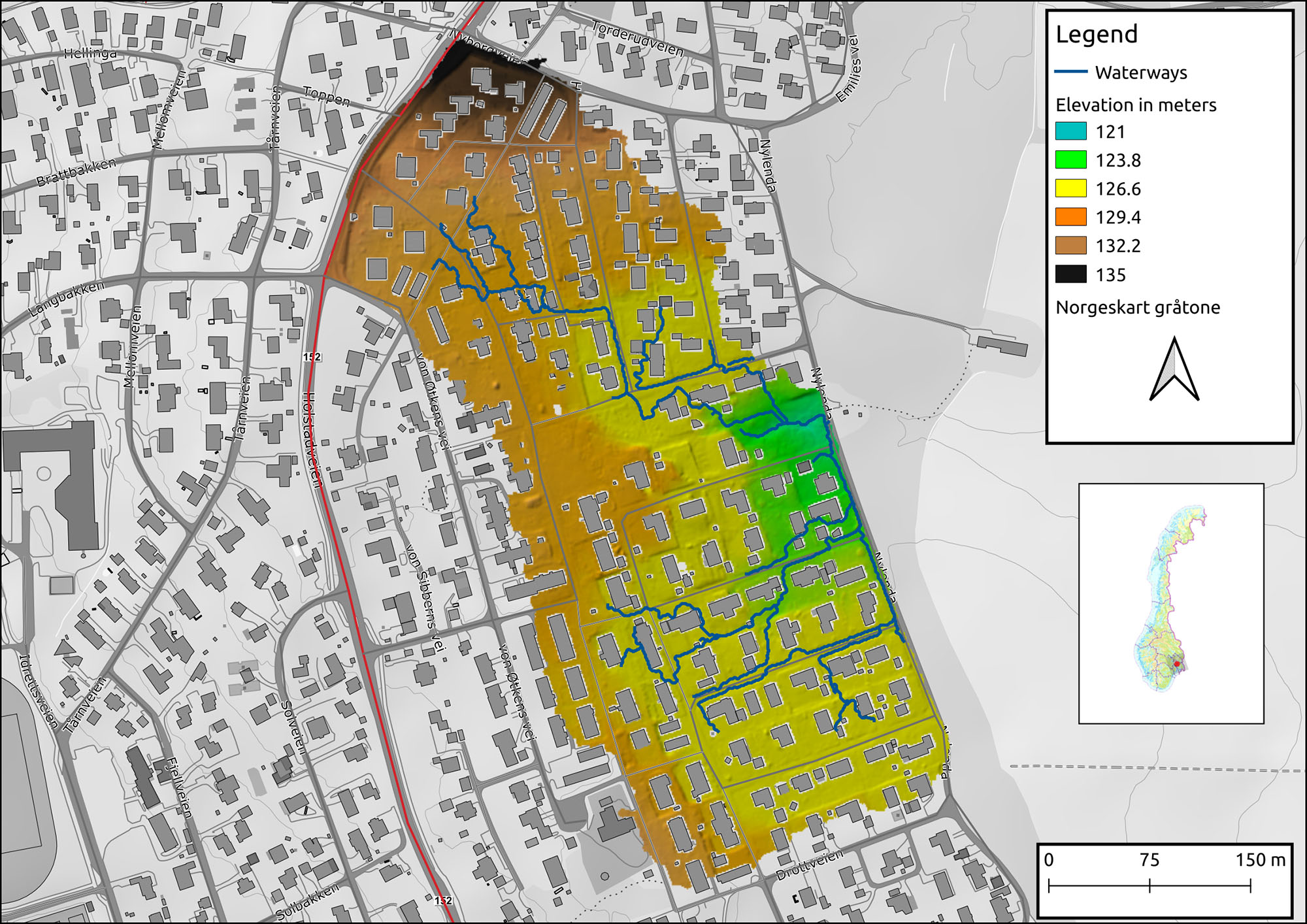
Figure 1.
Area of study.
Data and Software
Data
We use a digital terrain model (DTM) obtained from the Norwegian national topographic data server (Kartverket, n.d.-b.). This high-resolution DTM, with a one-meter resolution (DTM1), provides detailed information about the terrain and elevation of the study area.
In addition to the DTM, we incorporate surface permeability data. Two vector layers were acquired at Kartverket (n.d.-a). These layers contain information on the distribution of permeable surfaces (e.g., soil) and impermeable surfaces (e.g., buildings and roads) within the study area. We use the permeability data to determine Manning’s coefficient for further analyses.
PyGRASS
We use the PyGRASS Python package within a web-based interactive development environment called Jupyter notebook to conduct hydrological analyses. PyGRASS acts as an object-oriented Python API for the Geographic Resources Analysis Support System (GRASS Development Team, 2025; Zambelli et al., 2013). Specifically, we utilize the r.watershed, r.water.outlet, r.extract.stream and r.mask modules to delineate the watershed.
Itzï
Itzï (version 17.1) is a 2D hydrodynamic model developed by Courty et al. in 2017. Itzï uses a simplified form of the shallow water equations (SWE) and the damped partial inertia equation to simulate overland water flow infiltration. Itzï employs an explicit finite difference numerical scheme to solve the simplified SWE. This scheme is applied to a staggered 2D grid arrangement, where water depth and elevation are evaluated at the center of the cells, while water flow and velocity are evaluated at the cells’ faces.
To ensure model stability under subcritical flooding conditions, common in urban environments, De Almeida et al. (2012) introduced the adaptive stepping method, based on the standard Courant-Friedrichs-Lewy (CFL) condition. De Almeida et al. (2012) recommend a CFL value of 0.7 to optimize computation time while maintaining numerical stability. Itzï’s modular design enables seamless integration with third-party software, such as the Storm Water Management Model (SWMM), allowing for the evaluation of culvert impacts on simulated flood events. Itzï has been successfully used to model real-world flood events in the city of Kingston upon Hull in the United Kingdom (UK) (Courty & Pedrozo-Acuña, 2016).
R.sim.water
R.sim.water (Rsim) is a module within the SIMulated Water Erosion (SIMWE) framework, developed by Mitasova et al. at the University of North Carolina (Thaxton, C. S. et al., 2004). It simulates steady-state overland flow and infiltration using a stochastic approach. This means it incorporates randomness to account for the variability in real-world terrain and rainfall.
The model employs a combination of the Monte Carlo path simulation and the Green-Ampt equation to solve the SWE (Thaxton, C. S. et al., 2004). A key concept is the duality between the behavior of discrete particles and continuous fields. In Rsim, these particles are called walkers and represent individual water droplets. The continuous field, on the other hand, represents the terrain surface.
By applying the path sampling method, Rsim simulates the movement and decay of walkers across the terrain, effectively representing overland water flow (Thaxton, C. S. et al., 2004). The direction and speed of these walkers are determined by the second derivatives of slope and aspect of the terrain, derived from a DTM (Thaxton, C. S. et al., 2004).
Rsim has been successfully applied in urban environments of Norway to model overland flow and assess the effectiveness of green infrastructure solutions in managing stormwater (Bratlie, R. et al., 2023; Li et al., 2020; Ortega & Zanusso, 2022).
Fastflood
Fastflood (standard version, free of cost) is a steady-state overland flow model developed by the University of Twente (Van den Bout, B. et al., 2023b). It uses a multi-directional sweeping algorithm to efficiently calculate flow accumulation, which compares favorably to results from the Saint-Venant equations (Van den Bout, B. et al., 2023a). Unlike traditional methods that iterate over grid cells, Fastflood employs a minimal steady-state solver to determine stable flow direction and discharge.
This allows water to move quickly across large areas, as long as the flow direction remains consistent. Inverted accumulation values, derived from the Manning’s surface flow law (an inverse of kinematic flow momentum balance), and discharge are used to estimate flow depth (Van den Bout, B. et al., 2023a). The fast estimation of steady-state velocity fields linked with inverted flow-accumulation fields provides an extremely fast method for estimation of steady-state flow heights.
This efficiency makes Fastflood well-suited for web-based applications, lowering the barrier to entry for practitioners new to the field (Van den Bout, B. et al., 2023b). Fastflood has been successfully applied to model flood events in non-urban environments (Van den Bout, B. et al., 2023a). To the present knowledge of the authors, it has not yet been used in urban environments.
Flusstools
Flusstools (v1.1.8) is a Python package developed by the University of Stuttgart for fuzzy comparison of continuous valued raster datasets (Negreiros et al., 2022). By incorporating fuzzy spatial relationships, Flusstools enables more accurate comparisons of raster data, even when slight spatial misalignments exist. This approach accounts for the inherent imprecision in spatial data and improves the robustness of analyses (Negreiros et al., 2022; Hagen-Zanker, 2006). Fuzzy tolerance also accommodates algorithms with different input handling and parameter settings.
The concept of fuzziness of location in Flusstools means that a pixel in one simulated map can be considered similar not only to its exact counterpart in another map but also to neighboring pixels (Negreiros et al., 2022). To achieve this, Flusstools introduces the concept of fuzzy pixels, where the neighborhood of each fuzzy pixel is defined by a finite distance, called the neighborhood radius (rad). Rad represents a window of N pixels, including the central pixel (Negreiros et al., 2022).
The degree to which neighboring pixels contribute to the fuzzy representation of a central pixel is determined by a distance decay membership function (Negreiros et al., 2022; Hagen-Zanker, 2006). This function involves the use of the halving distance (dhalv), which is the distance in pixels at which the membership function decays to half its maximum value at the central pixel (Negreiros et al., 2022; Hagen-Zanker, 2006) (Figure 2).

Figure 2.
Qualitative example for introducing fuzziness of location through a fuzzy pixel with a neighborhood radius (Rad) of one pixel (total number of neighboring pixels N = 9) and an exponential distance decay membership function ω(dij, ι, dhalv) with a halving distance (dhalv) of one pixel. dij, ι is the distance between the neighboring pixel and the central pixel at ij. Printed with permission of Negreiros et al., 2022.
Method
This investigation consists of five distinct parts:
-
Creating a hybrid DTM
-
Delineation of watershed and generation of water ways using hydrological analysis
-
Calculation of a single urban flood event using Itzï, Rsim and Fastflood algorithms
-
Evaluation of the depth and velocity raster layers using a numerical fuzzy map comparison method
-
Calculation and evaluation of the depth–velocity number (DV number) for each model
Create a Hybrid DTM
To account for the influence of urban patterns, such as roads and buildings, on overland flow modeling, we utilize the v.extrude module in GRASS GIS. This module transforms the 2D layer representing house roofs into 3D features by assigning specific elevation values to each vertex of the extruded features using the elevation parameter (GRASS Development Team, 2025). The result is a hybrid DTM that incorporates buildings as 3D features in the overland flow modeling.
Delineation of the Watershed Using Hydrological Analysis
We employ GRASS GIS to delineate the study area watershed using a DTM1. We utilize the r.watershed module to calculate flow accumulation, flow direction, and stream lines. Subsequently, We use the r.water.outlet module in conjunction with the x and y coordinates of the RURS point to determine the extent of the watershed. Finally, We use the r.stream.extract to create the waterways vector and the r.mask module to create watershed boundary mask for subsequent analyses (GRASS Development Team, 2025)
Calculation of a Single Urban Flood Event Using Itzï, Rsim and Fastflood Algorithms
To model a single urban flow event using the three algorithms described in the software section, I employ the following inputs and parameters:
-
Hybrid DTM with 1 meter resolution
-
Two raster layers containing Manning’s roughness coefficients for permeable and impermeable surfaces
-
54 millimeters (mm) of precipitation based on a 2-year extreme value precipitation observed by Storteig, I. et al., during the 25 -years precipitation time series analysis performed for RURS
-
A simulation time of 60 minutes
The modeling process involved two steps. The Itzï and Rsim modules were executed within GRASS GIS, while the Fastflood algorithm was run on a web-based application optimized for its specific functionality (Van den Bout, B. et al., 2023b). In all three cases, infiltration is not considered due to lack of information. Manning coefficients are 0.5 for impermeable surfaces and 0.25 for permeable surfaces.
Evaluation of the Depth and Velocity Raster Layers Using a Numerical Fuzzy Map Comparison Method
To evaluate the performance of the flood modeling algorithms, we employ Flusstools to compare the generated water depth and velocity raster maps. For this study, we selected a radius (rad) of eight meters, which is twice the width of the local roads in the study area, and a half-distance (dhalv) of four meters, representing the approximate road width (Figure 3). While the fuzzy map comparison evaluates the entire raster, the roads, buildings, and their neighboring areas are of particular interest in urban flood modeling. This is because the spatial heterogeneity of roads and buildings, also known as the urban pattern, significantly influences overland flow patterns.
Calculation and Evaluation of the Depth–Velocity Number (DV Number) for Each Model
The DV number is the direct multiplication of the water’s depth and its velocity (D * V). It provides a basic measure of the momentum and force of flowing water. It is primarily used for assessing flood hazard severity and helps determine the potential for floodwaters to cause damage or pose a risk to safety. We calculate the DV number using the D and V simulated by each of the models and evaluate them visually to determine differences in the dimension and spatial distribution of the DV number.
Results
To better highlight the findings in this research, we partition the area of study into three areas: an upper Area A, with the highest elevations; a lower Area B, with the flattest landscape; and an Area C, with the lowest elevations, including the outlet (Figure 4). This partition allows to better understand of the different degree of similarity exhibited by models as a response to the location across the landscape
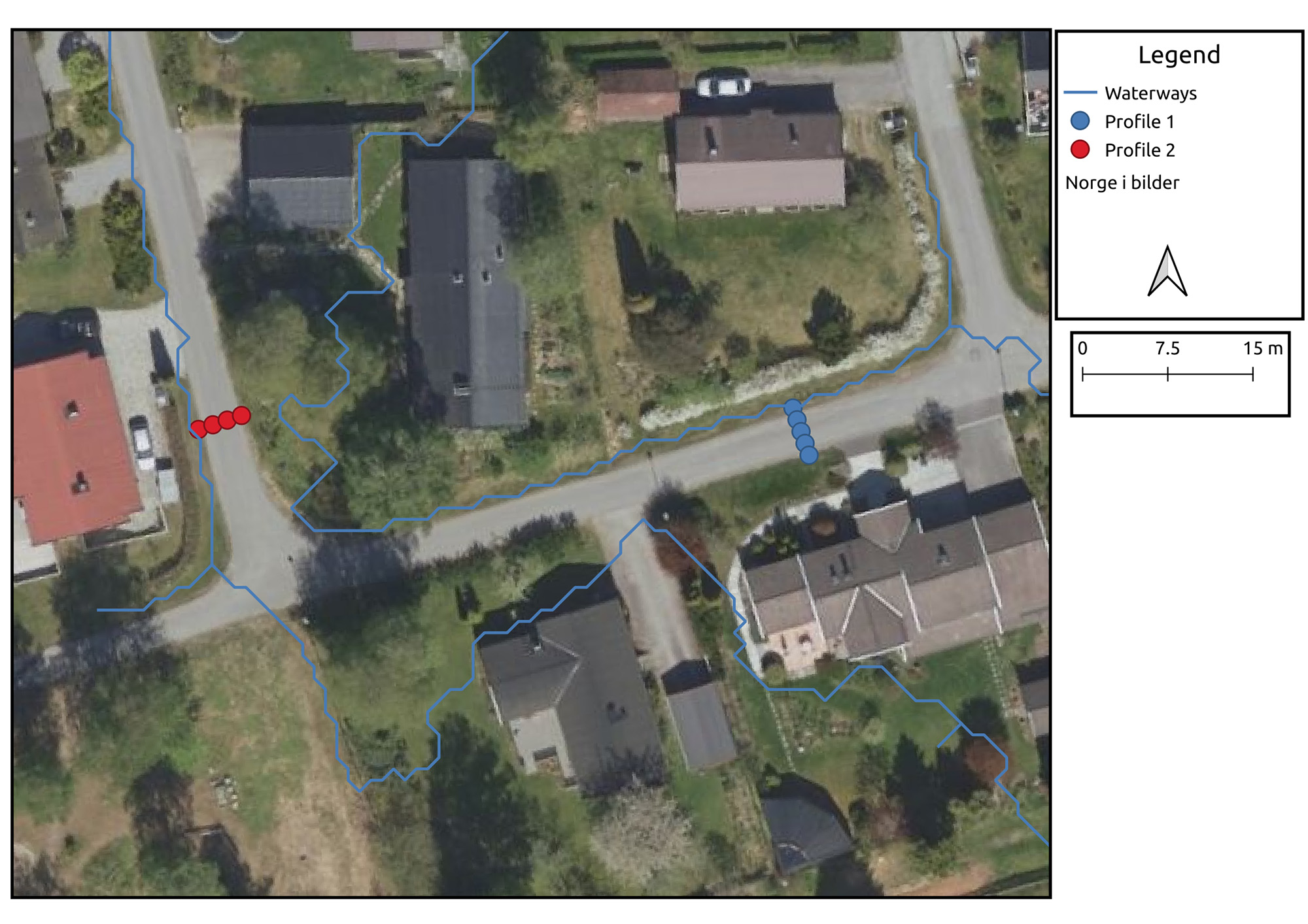
Figure 3.
Example of measurements profiles, to determine the width of the local roads, used as dhalv parameter in exponential distance decay membership function.
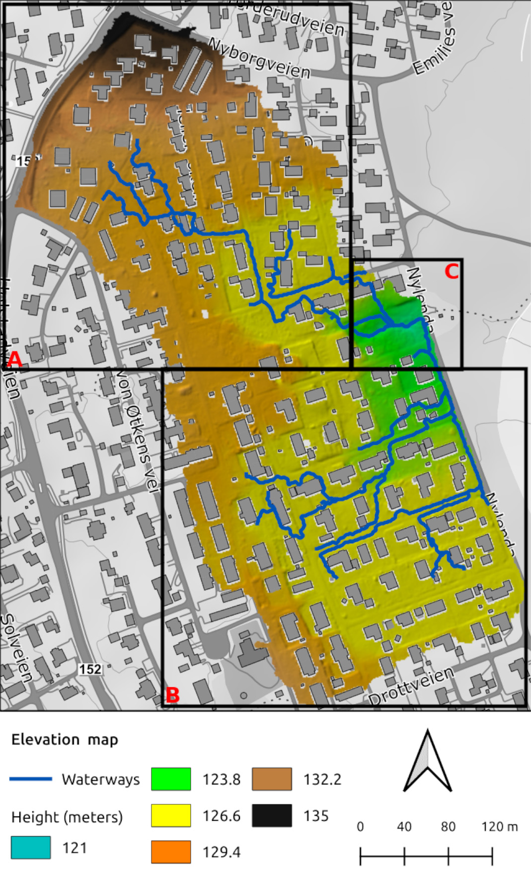
Figure 4.
Partition of the area of study: upper Area A, with the highest elevations, lower Area B, with the flattest terrain, and Area C, with the lowest elevations and the flood culmination site.
Fuzzy Numerical Map Comparison of the Water Depths
The results of the depth and velocity raster comparison using the fuzzy numerical approach shows that Itzï and Rsim have the highest probability of similarity (0.59). The lowest probability of similarity occurs between Rsim and Fastflood (Table 1).
Table 1.
Average fuzzy similarity (water depth) | Probability |
|---|---|
Itzï vs Rsim | 0.59 |
Itzï vs Fastflood | 0.49 |
Rsim vs Fastflood | 0.43 |
A visual comparison of water depth rasters in Figure 5 shows that Fastflood and Itzï produce more similar water flow patterns than Itzï and Rsim. However, further analysis of results of the depth raster comparison using histograms (Figure 6) confirm the quantitative findings in Table 1, providing additional insights into the probability distribution of water depth modeling across Areas A, B, and C.
The probability distribution for the Itzï–Rsim comparison, shown in Figure 6, indicates that the two models produce similar water depth results. The left-skewed distribution suggests that most raster cells in Areas A and B—except for the outlet (Area C)—have similarity values clustered toward the higher end of the scale, closer to 1.0, reflecting strong agreement between the models.
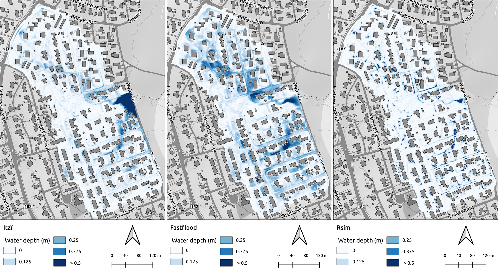
Figure 5.
Visual comparison of the modelled water depth pattern for Itzï (left), Fastflood (centre) and Rsim (right).
In contrast, the Itzï–Fastflood and Fastflood–Rsim comparisons reveal that approximately 10,800 cells exhibit non-similarity, accounting for about 2.8% of the total surface area (i.e., the total number of cells for the entire raster are 385714). These low-similarity regions are primarily located near houses, roads, and raster borders. The discrepancies stem from the Fastflood model, which uses a multi-directional sweeping approach to simulate water accumulation over large areas. While efficient, this method struggles with abrupt slope changes, a common feature in urban environments, leading to reduced accuracy in those zones.
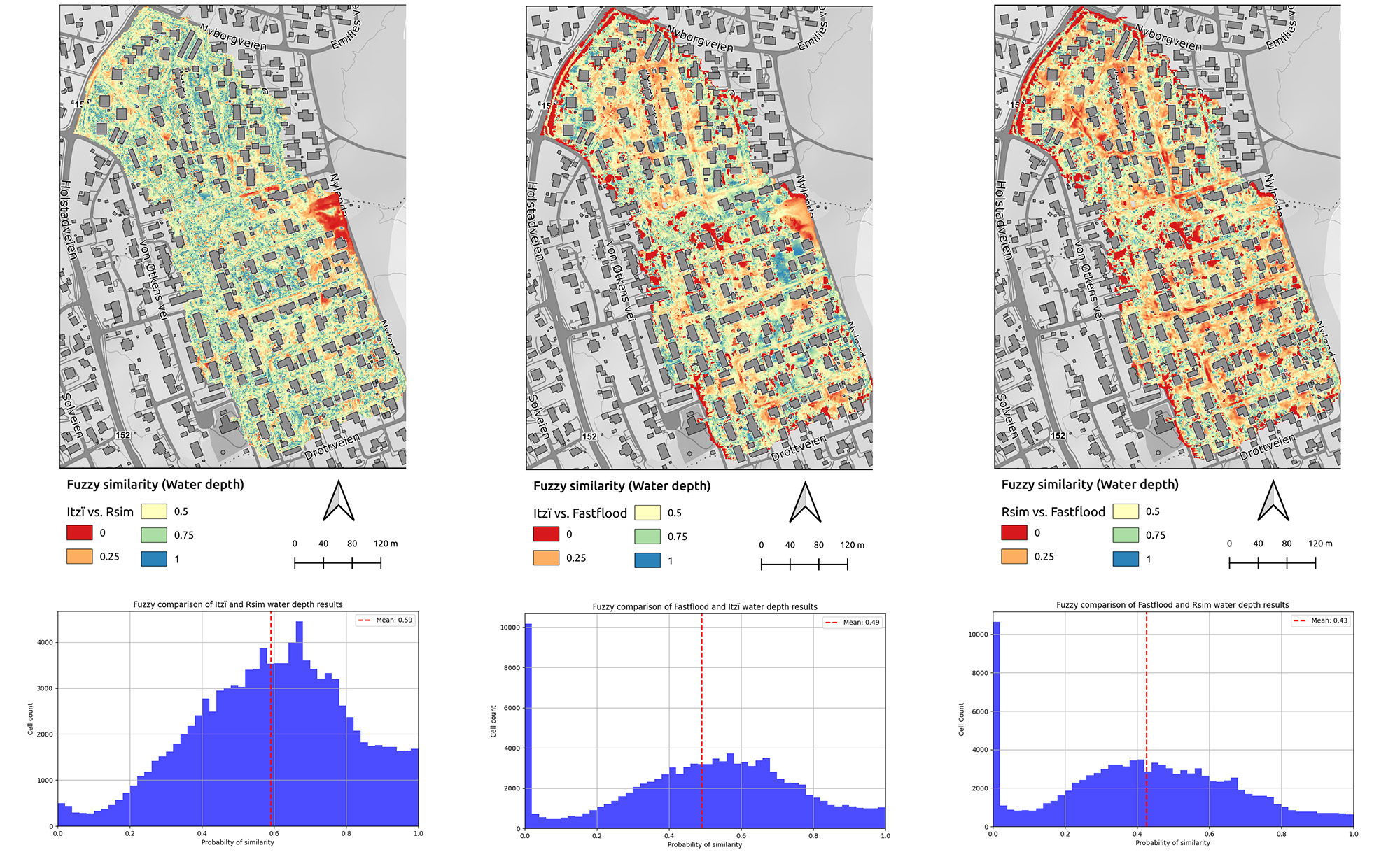
Figure 6.
Water depth fuzzy comparison of raster maps of Itzï, Fastflood and Rsim, together with the cell count distribution of probability of similarity, across the entire area of study. The similarity between water depth results is expressed as probability. With 0 in red and 1 in blue.
In both comparisons, the histograms display a right-skewed, asymmetrical shape, with a significant number of cells showing low similarity values (close to 0). Nonetheless, the peak of the distribution is centered around a similarity value of approximately 0.49, indicating that most cells still exhibit moderate agreement between the models.
Fuzzy Numerical Map Comparison of the Water Velocities
The comparison of velocities between Rsim and Fastflood shows the highest mean probability of similarity (0.53), followed by Itzï and Fastflood with average probability of similarity of 0.52. The lowest score shows between Itzï and Rsim with a probability of similarity of 0.44 (Table 2).
Table 2.
Mean fuzzy similarity (water velocity) | Probability |
|---|---|
Rsim vs. Fastflood | 0.53 |
Itzï vs Fastflood | 0.52 |
Itzï vs Rsim | 0.44 |
The depth–velocity relationship at the outlet (Area C) reveals a consistent trend between Rsim and Fastflood. Both models show an increase in water velocity with increasing depth. Rsim demonstrates a near-linear correlation, while Fastflood, despite exhibiting some degree of random variation, maintains a similar overall trend. Itzï’s results in Area C diverge significantly from Rsim and Fastflood, indicating an inverse relationship where water velocity decreases as depth increases. This observation is further supported by the velocity–depth panel charts in Figure 7.
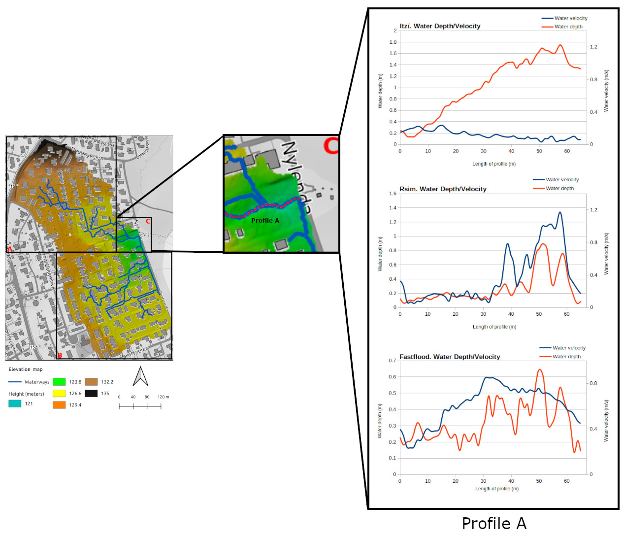
Figure 7.
Profile A at flood culmination site, Area C. Panel charts show water depth and velocity for Itzï, Rsim, and Fastflood.
Figure 8 presents a visual comparison of water velocity rasters generated by three models: Rsim, Fastflood, and Itzï. Rsim predicts notably higher water velocities in ponding zones across Areas A and B, suggesting a strong sensitivity to localized water accumulation. Fastflood also indicates elevated velocities in these regions, though to a lesser degree. Its velocity increases are primarily concentrated near buildings and at the outlet (Area C). In contrast, Rsim highlights additional velocity increases in smaller impoundments along roads, intersections, and within Area C.
Itzï, however, exhibits a distinct pattern. It identifies ponding primarily at the outlet (Area C) and near buildings in Area B, while uniquely predicting a decrease in water velocity with increasing depth. This inverse relationship, not observed in the other models, suggests that Itzï may offer a more realistic representation of overland flow dynamics, particularly in areas with significant water accumulation.
Further spatial insight is gained from the raster maps comparison for water velocities. The cell count distribution of similarity probabilities (Figure 9) complements the numerical results in Table 2. While a substantial number of cells indicate dissimilarity, the Itzï–Fastflood comparison shows higher overall similarity compared to Itzï–Rsim. Furthermore, Rsim and Fastflood exhibit the greatest similarity to each other, reinforcing their closer alignment in water velocity prediction.

Figure 8.
Visual comparison of the modelled water velocity pattern for Itzï (left), Fastflood (centre), and Rsim (right).

Figure 9.
Water velocity fuzzy comparison of raster maps of Itzï, Fastflood, and Rsim, together with the cell count distribution of probability of similarity, across the entire area of study. The similarity between water velocity results is expressed as probability. With 0 in red and 1 in blue.
DV Number Evaluation in Itzï, Rsim, and Fastflood
The depth–velocity (DV) number demonstrates significant variability across different models, primarily driven by variations in velocity and depth inputs. This variability directly influences both the assigned susceptibility levels and the spatial delineation of susceptible areas, ultimately affecting the perceived safety of those areas. Furthermore, the DV number is sensitive to modeled flood patterns. Notably, models with similar flow patterns exhibit comparable DV numbers, even when water velocity and depth inputs differ substantially (Figure 10). While Itzï and Fastflood show consistent potential flow hazard categories, Rsim tends to either underestimate or overestimate these hazards. Despite these differences, all three models display spatial variability in high and medium DV numbers.
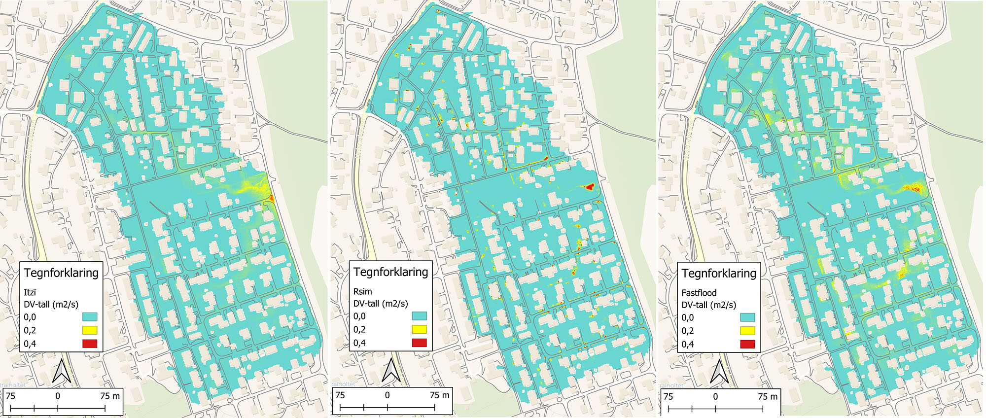
Figure 10.
Illustrating the DV number for Itzï, Rsim, and Fastflood. Values are expressed in m²/s. Gray indicates low potential for flood hazard, orange indicates medium potential for flood hazard, and red indicates high potential for flood hazard.
Discussion
This study presents a comparative fuzzy numerical evaluation of three overland flow models—R.sim.water (Rsim), Fastflood, and Itzï—in the context of the newly amended Norwegian Building Regulations, which emphasize effective stormwater management. The analysis focused on the Rustadskogen urban area in Ås municipality, Norway, utilizing a comprehensive 25-year precipitation dataset from RURS. A fuzzy map comparison method was employed to address the current gap in comparative performance assessments of these models within the Norwegian context, particularly regarding their ability to simulate water depth, velocity, and the derived depth–velocity (DV) number.
Water Depth
Itzï and Rsim demonstrated the highest average fuzzy similarity in water depth predictions, suggesting a close alignment in their outputs. However, visual inspection of the depth rasters revealed that Fastflood and Itzï shared more similar spatial patterns. This discrepancy underscores the importance of integrating both quantitative and qualitative assessments in model evaluation. Histogram analyses of the fuzzy comparison rasters further supported these findings, showing that Areas A and B had higher similarity between Itzï and Rsim, while Area C (the outlet) exhibited greater variability.
Water Velocity
Rsim and Fastflood showed the highest average fuzzy similarity in velocity predictions, followed by Itzï and Fastflood. This suggests that Fastflood’s velocity outputs align more closely with both models. However, the depth–velocity relationship at the outlet (Area C) revealed a significant divergence in Itzï’s results. While Rsim and Fastflood showed increasing velocity with depth, Itzï exhibited an inverse relationship, indicating a potentially more realistic representation of overland flow dynamics in areas with significant water accumulation. Visual comparisons of velocity rasters highlighted further differences:
-
Rsim predicted elevated velocities in widespread ponding areas
-
Fastflood showed localized increases near buildings and the outlet
-
Itzï displayed ponding primarily at the outlet with velocity decrease and depth increase and near buildings in Area B
Depth–Velocity (DV) Number
The DV number, a key indicator for flood hazard assessment, varied significantly across the models. These differences were primarily driven by variations in depth and velocity inputs, which influenced the spatial distribution of susceptibility levels. Despite these differences, models with similar flow patterns tended to produce comparable DV numbers. Notably, Itzï and Fastflood showed consistent hazard classifications, while Rsim tended to underestimate or overestimate flood hazards.
Methodological Insights
The fuzzy map comparison approach proved effective in accounting for spatial uncertainty and quantitative inaccuracies. The use of a radius (rad) of eight meters and half-distance (dhalv) of four meters, based on local road widths, enabled a focused evaluation of model performance in urban flood-prone areas such as roads. Dividing the study area into three zones (A, B, and C) allowed for a more nuanced understanding of model behavior across varying terrain types.
Implications and Future Work
These findings have important implications for the implementation of the Norwegian Building Regulations. The comparative evaluation provides valuable insights into the strengths and limitations of each model, supporting informed decision-making in stormwater management planning and design. The study also highlights the value of combining quantitative metrics with visual assessments, and the need to account for spatial uncertainty in model evaluation.
Future research should explore:
-
Sensitivity analyses to input parameters (e.g., precipitation intensity, duration, Manning’s coefficients)
-
Infiltration modeling for a more comprehensive hydrological representation
-
Validation with real-world flood events
-
Assessment of computational efficiency and scalability for larger urban area
Conclusion
This study conducted a comprehensive fuzzy similarity analysis of three overland flow models—Rsim, Fastflood, and Itzï—within the framework of updated Norwegian Building Regulations that emphasize effective stormwater management. By applying a fuzzy map comparison method to a 25-year precipitation dataset in the Rustadskogen urban area, the research revealed significant differences in model performance related to water depth, velocity, and the derived depth–velocity (DV) number.
The results showed that while Rsim and Fastflood had higher average similarity in velocity predictions, Itzï demonstrated a more realistic depth–velocity relationship, particularly in areas with substantial water accumulation. In terms of water depth, Itzï and Rsim aligned quantitatively, but Fastflood and Itzï shared more similar spatial patterns. These findings underscore the importance of combining quantitative metrics with visual assessments to fully understand model behavior.
The DV number analysis further highlighted variability in flood hazard predictions, with Itzï and Fastflood offering more consistent classifications than Rsim. The fuzzy comparison approach proved valuable in accounting for spatial uncertainty and enhancing model evaluation in urban flood contexts.
Overall, this study provides actionable insights for selecting appropriate hydrological models in urban planning and stormwater design. Future research should focus on model sensitivity to input parameters, integration of infiltration processes, validation with real flood events, and scalability for larger urban areas.
Acknowledgements
The authors would like to thank Thomas Skaugen (NVE), Rune Bratlie (Multiconsult AS) and Rhonald Ortega (University of North Carolina) for their valuable contributions to this work. Their support in proofreading the manuscript and providing insightful ideas greatly enhanced the quality of the research.
References
-
Bratlie, R.,Fleming, C.,Holsdal, I.,Ortega, R.,Rasten, B.,andBorsányi, P.(2023).
Klimasårbarhetsanalyse for Drammen kommune (Dokument 10246790-01-RIVA-RAP-001)
.Multiconsult AS
. Retrieved April 30, 2023, from https://www.miljodirektoratet.no/ansvarsomrader/klima/for-myndigheter/klimatilpasning/klimatilpasning-prosjekter/2022/klimasarbarhetsanalyse-for-drammen-kommune/ -
Courty, L. G.,andPedrozo-Acuña, A.(2016). A GRASS GIS module for 2D superficial flow simulations. In
Proceedings of the 12th International Conference on Hydroinformatics
(Vol. 10). -
Courty, L. G.,Pedrozo-Acuña, A.,andBates, P. D.(2017). Itzï (version 17.1): An open-source, distributed GIS model for dynamic flood simulation.
Geoscientific Model Development
, 10(4), 1835–1847. -
De Almeida, G. A.,Bates, P.,Freer, J. E.,&Souvignet, M.(2012). Improving the stability of a simple formulation of the shallow water equations for 2‐D flood modeling.
Water Resources Research
, 48(5). -
GRASS Development Team. (2025).
Geographic Resources Analysis Support System (GRASS GIS) Software, Version 8.2
[Computer software]. Open Source Geospatial Foundation.
https://doi.org/10.5281/zenodo.5176030 -
Hagen, A.(2006) Comparing continuous valued raster data: A crossdisciplinary literature scan, Technical report.
Maastricht
:ResearchInstitute for Knowledge Systems (RIKS)
. -
Kartverket. (n.d.-b).
LaserInnsyn
.Høydedata.no. Retrieved September 24, 2024, from
https://hoydedata.no/LaserInnsyn2 -
Kommunal- og distriktsdepartementet. (2022).
Prop. 125 L (2021–2022): Endringar i plan- og bygningsloven (reglar om handtering av overvatn i byggjesaker mv.)
.Regjeringen.no. Retrieved December 15, 2024, from
https://www.regjeringen.no/no/dokumenter/prop.-125-l-20212022/id2916622/ -
Li, H.,Gao, H.,Zhou, Y.,Xu, C. Y.,Ortega M,R. Z.,andSælthun, N. R.(2020). Usage of SIMWE model to model urban overland flood: a case study in Oslo.
Hydrology Research
, 51(2), 366–380. -
Negreiros, B.,Schwindt, S.,Haun, S.,andWieprecht, S.(2022). Fuzzy map comparisons enable objective hydro-morphodynamic model validation.
Earth Surface Processes and Landforms
, 47(3), 793–806. -
Ortega, R.,andZanusso, E.(2022). Planning green infrastructure in dense urban areas with the Tangible Landscape (TL): A case study of the re-opening of the Mærradal creek in the city of Oslo, Norway.
Kart og Plan
, 115(4), 382–399. -
Pedersen, T. B.,Bratlie, R.,Verbaan, I. J.,Sandal, B.,Solbrå, S. T.,Hagerup, T. G.,Röttorp, A. M.,Fleig, A.,Stickler, M.,Sommer-Erichson, P. E.,Dalen, E. V.,Storteig, I. C.,Tvedalen, K.,Dören, L. W.,&Langsjøvold, S. J.(2022).
Korleis ta omsyn til vassmengder? NVE Veileder nr. 4/2022: Rettleiar for handtering av overvatn i arealplanar
.Norges vassdrags- og energidirektorat (NVE).
-
Skaugen, T.,Lawrence, D.,andOrtega, R. Z.(2020). A parameter parsimonious approach for catchment scale urban hydrology–Which processes are important?.
Journal of Hydrology X
, 8, 100060. -
Storteig, I.,Skaugen, T.,andOrtega, R. Z.(2023).
Simulering av NVEs urbanfelt med urbanhydrologisk nedbør-avløpsmodell (DDDUrban)
.Norges vassdrags- og energidirektorat (NVE).
-
Thaxton, C. S.,Mitasova, H.,Mitas, L.,andMcLaughlin, R.(2004). Simulations of distributed watershed erosion, deposition, and terrain evolution using a path sampling Monte Carlo method. In
2004 ASAE Annual Meeting (p. 1). American Society of Agricultural and Biological Engineers
. -
Van den Bout, B.,Jetten, V. G.,van Westen, C. J.,andLombardo, L.(2023a). A breakthrough in fast flood simulation.
Environmental Modelling and Software
, 168, 105787. -
Van den Bout, B.,Jetten, V.,van Westen, C.,andLombardo, L.(2023b).
Fastflood.org: An open-source super-fast flood model in the browser
.University of Twente
https://doi.org/10.5194/egusphere-egu23-3611, 2023 -
Zambelli, P.,Gebbert, S.,andCiolli, M.(2013). Pygrass: An object-oriented python application programming interface (API) for geographic resources analysis support system (GRASS) geographic information system (GIS).
ISPRS International Journal of Geo-Information
, 2(1), 201–219.